Regression Model Of Household Consumption Expenditure Coursework

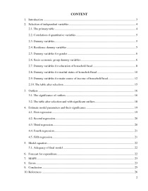
Introduction. Selection of independent variables. The primary table. Correlation of quantitative variables. Dummy variables. Residence dummy variables. Dummy variables for gender. Socio economic group dummy variables. Dummy variables for education of household head. Dummy variables for marital status of household head. Dummy variables for main source of income of household head. The table after selection. Outliers. The significance of outliers. The table after selection and with significant outliers. Estimate model parameters and their significance. First regression. Second regression. Third regression. Fourth regression. Fifth regression. Model equation. Adequacy of final model. Forecast for expenditure. Mape. Errors. Conclusion. References.

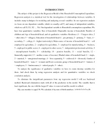
My case number is equal 36. We calculate it by sum of birth numbers:

I checked the significance of quantitative variables by using correlation analyze.

From the table 2 we can see that significant is only disposable income of household, because its correlation is more than 0.5. We can delete all other quantitative variables. Also we should check multicollinearity, if some of variables do not have similar values. We can see it in third, fourth and fifth columns then correlation index is higher than 0.8. We do not have multicollinearity in this case.

If we want to check the significance of qualitative variables, the have to change them into dummy variables, which have only two values: 1 if it fits the new variable and 0 if it does not. When we create dummy variables we have to use one less values.

Firstly I created dummy variables for Residence: 5 largest cities and villages, and checked their significance by using regression model. Both, 5 largest cities and villages are insignificant because their significance F (p value) is more than 0.05: I am going to remove them.

Also I created dummy variables for gender, as a new variable I used man, but this variable was not significant, and I deleted it.

Further I created the variables for socio economic group: farmers, employees, businessmen and retired people. I deleted the farmers because all values of this new variable were equal to 0. The significance I found in retired people:

I created the variables for education of household head: pre – primary, primary, basic, secondary, college. The significance I found in household head which had college education.

I created the variables for marital status of household head: single, married, unregistered marriage, lives separately, widowed. The significance I found in married status.

2.9. Dummy variables for main source of income of household head

I created the variables for main source of income of household head: self employed in agriculture, employed in agriculture, employed in manufacturing, business, employed in public sector, employed in other sector, independent professional activities, unemployment benefits, scholarship, pension benefits, social benefits, financially supported. I deleted employed in agriculture, independent professional activities, unemployment benefits, scholarship and financially supported variables because all values of those new variables were equal to 0. The significance I found in pension benefits.

We already have six significant variables, we can choose not to check others, and simply delete them. And our table looks like (Table 26):

To check the possibility of significant outliers, firstly we have to scatter plot our dependent variable – Household consumption expenditure. Because some of the values, which are outliers, can have a significance to our model equation.